Eigenfunctions and energy levels of a quantum particle in an infinite square well
Posted on
In this post, we will explore the solutions to the standard quantum mechanics problem of a particle trapped in a 1D box, or infinite square well. We'll first have a look at how to derive these solutions, and then see what the solutions look like, thanks to interactive graphs.
Derivation
We are looking for the energy eigenvalues and energy eigenfunctions of the particle. Here's the standard recipe that we will apply in order to obtain these solutions:
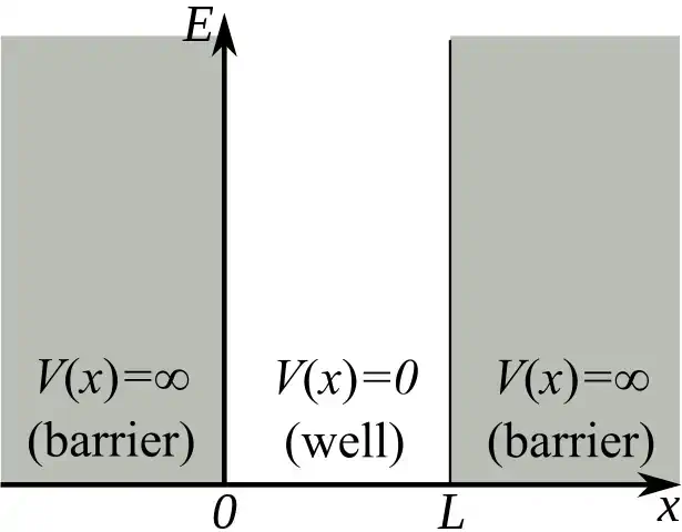
Specifying the potential
For a particle trapped in an infinite square well, the potential energy \(V\) is:
The potential energy is shown in the following graph:
Now that our potential is set up, we can move on to the next step!
Applying the time-independant Schrödinger equation
The time-independant Schrödinger equation is the form of the Schrödinger equation that we will use here to find the energy eigenvalues \(E_n\) and energy eigenfunctions \(\psi_n\) of the trapped particle. We start with:
And insert the potential energy \(V\) that we previously specified. We get the following, for the region inside the well \(0\le x\le L\):
This can be rearranged as:
This is a standard differential equation for which the general solutions are:
It's now time to make use of the well's boundary conditions!
Using boundary conditions
Boundary conditions are the values that we expect for wavefunctions at the edges of the well. Because the potential is infinite at \(x=0\) and \(x=L\), the particle can not possibly be found at the well's edges. We get:
This means that the eigenfunctions can not contain a cosine term, so \(B=0\). We also deduce that \(k_n=\frac{n\pi}{L}\) . Equating this with our previous formula for \(k_n\) gives us the energy eigenvalues.
Normalization of the eigenfunctions
Normalization is a recurring technique in quantum mechanics to find the coefficients of eigenfunctions. As we know, \(|\psi|^2\) is a probability density function. This means that integrating over all values of x must equal to 1.
So the eigenfunctions are:
Let's now have a look at the solutions we just derived!
Visualisation of the solutions
Let's now have a look at the solutions thanks to a couple graphs.
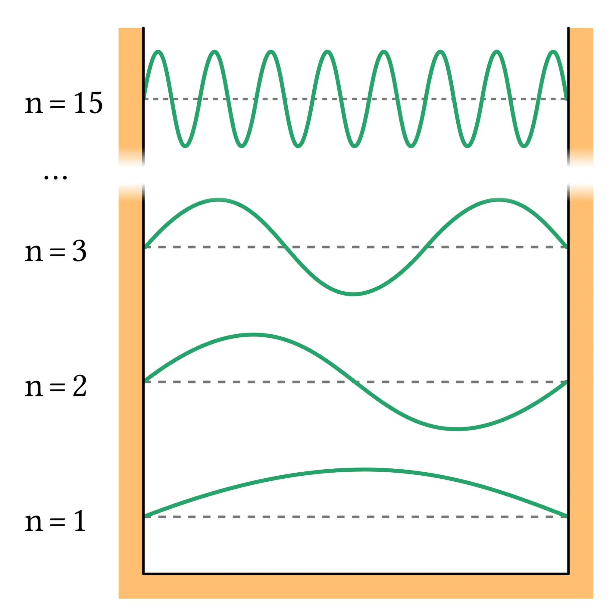
Energy eigenfunction
Here's a graph showing the energy eingenfunctions of a quantum particle in a 1-dimensional box. Use the sliders to modify the quantum number and the length of the well.
Superposition states
Valid wavefunctions in the well can be made up of a sum of energy eigenfunctions. A state obtained in such a way is called a superposition state. Note that it is important to normalize superposition states, in the same way as we normalized base states.
The graph below shows the wavefunction resulting from the superposition state of three base states of different amplitudes.
That's it for today! You can explore time-dependance of wavefunctions in the infinite square well in this post.