Time evolution of wavefunctions in a harmonic oscillator
Posted on
We've all seen graphs of the first few eigenkets in the quantum simple harmonic oscillator, but how do pure and superposition state wavefunctions evolve with time in a SHO potential? Let's see!
We'll first have a look at the time-independant solutions, a necessary step before diving deeper. Then, we'll see how eigenfunctions evolve with time, and finish with the most interesting case, the time dependance of superposition states.
Time-independant solutions
The classical simple harmonic oscillator is characterised by a Hooke's law potential:
With \(k\) the spring constant. Simple harmonic oscillators are often studied in classical physics through pendulums and springs. The quantum version of such an oscillator has the same potential, usually rewritten as:
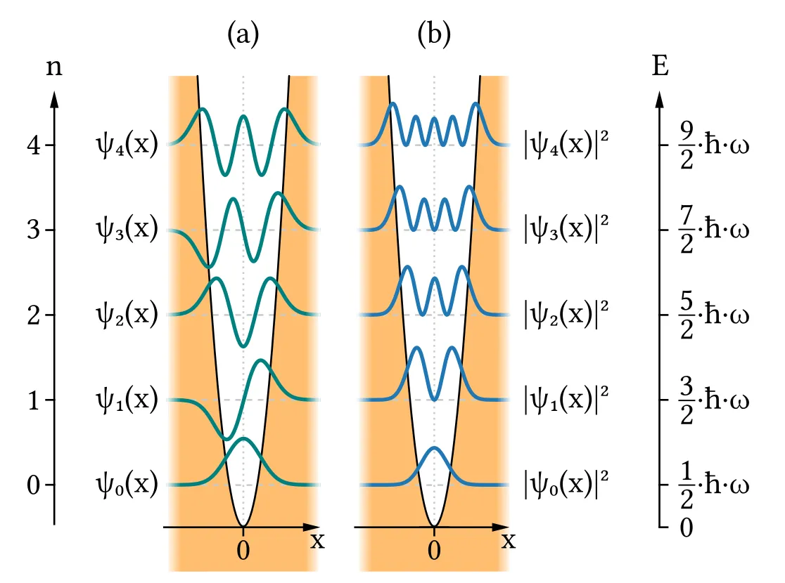
With angular frequency \(\omega\). One can use the Schrödinger equation to find the energy eigenvalues \(E_n\) and eigenfunctions \(\psi_n\) of this potential. The energy eigenvalues have a beautifully simple formula:
There is something remarkable about this: energy levels in the quantum harmonic oscillator are evenly spaced, with a separation of \(\hbar\omega\).
However, we're not so lucky with energy eigenfunctions, there's no analytical solution for them. But fear not! There's a relatively simple recurrence relation for them that uses ladder operators:
\(A\) is the so-called raising operator, with formula:
Starting from the ground-state wavefunction and using the formulae above, we can calculate the first few energy eigenkets:
It's important to note that every even eigenket is an even function, and every odd eigenket is odd. This is actually a property of symmetric potentials, which is also the case of the infinitely deep square well!
The first few eigenket are displayed in the graph below.
We can now move on to time considerations!
Time evolution of eigenkets
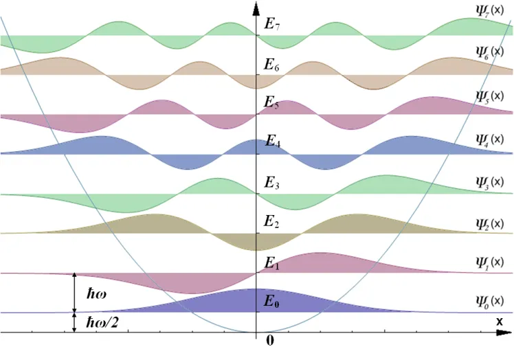
As always, probability density functions that describe base states are independant of time. But it doesn't mean that energy eigenfunctions themselves don't vary with time! Their factor of \(e^{-i\frac{E_n}{\hbar}t}\) makes them complex functions, with real and complex parts that oscillate with time. The following graph shows what it looks like:
In the graph above, \(x_0\) stands for the natural length of the harmonic oscillator, with formula:
You can see that the higher the excited state, the faster the oscillation! This is due to the fact that energy eigenvalues \(E_n\) grow linearly with \(n\). However, in comparison, eigenkets in the infinitely deep square well oscillate much faster, due the factor of \(n^2\) in the energy eigenvalues of the well. You can compare the oscillation of eigenkets in the harmonic oscillator with the time-dependance of eigenkets for a particle in a box.
We can now have a look at superposition states.
Superpositions
Superposition states are a normalized sum of eigenkets, with potentially different coefficients for each eigenket. For example, a simple superposition state \(|\psi\rangle\) could be made with an equal weight of \(|\psi_0\rangle\) and \(|\psi_1\rangle\)
To find the time-dependance of superposition states, just add to each eigenket a factor of \(e^{-i\frac{E_n}{\hbar}t}\). For our superposition state \(\psi\) in a harmonic oscillator, this results in:
Using this, we can obtain the time-dependance of the probability density function that represents that state:
Where we can replace the ugly coefficient on the right using the exponential form of cosine to get:
A much nicer equation! This shows that time-dependant terms in probability density functions come from cross-factors between different eigenkets.
Using this knowledge, we can plot the time-dependance of superposition states in a harmonic oscillator:
Feel free to play around and experiment with the controls. Remember that higher values of the probability density function in a certain area represents a higher chance to find the particle in that area.